- The growing and more rigorous application of standard VaR measures in the investment industry creates a systemic risk.
- Individual investors as well as the stability of markets are better off with VaR measures that do not overreact to recent large price moves.
- Using lower moment estimators for higher moment statistics is one of the ways to accomplish this.
In the past two decades, Value-at-Risk (VaR) measures have become popular tools for risk analysis of, among others, investment products. One of their great features is that independent risk monitors can apply them in a uniform way for completely different investments. This makes different investments comparable. But in this uniform approach lies the pitfall. A standard approach is typically not suited for more extreme circumstances. This weakness becomes very relevant if one does not only use VaR for evaluation purposes, but also as an investment management tool.
One of the main weaknesses of standard VaR measures is their overreaction to recent large price moves. As an example, Graph 1 shows the VaR history in 2015 of one of our funds managed pursuant to our Diversified Trend Program (DTP). The orange line is a generally accepted standard VaR statistic calculated by the fund’s independent risk reporting agent. The backbone of DTP’s risk management has always been an extreme risk measure. Derived from this measure we calculate a tailor made VaR, which we call exVaR. The blue lines in the graph show the 95% and the 99% exVaR for the same fund.
Graph 1: Various Value-at-Risk measures in perspective
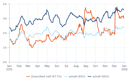
If the VaR and exVaR measures would be comparable, the orange 97.7% VaR should always be somewhere in the middle between the two blue lines. In reality, it is not. Most of the time the orange curve is significantly below that level, meaning that the exVaR measures a much higher risk – up to two times higher – than the standard VaR. Only on two occasions the VaR peaked significantly above that; the first time during the whole month of September and the second time in December.
The sharp rises of the standard VaR followed immediately after large price moves. On 11 August, the Chinese renminbi was devaluated. This caused a first steep rise in VaR, followed by a comparable fall after six weeks, in the second half of September. A steeper rise in VaR took place in the last week of August, following the 24th (China’s 'Black Monday'). The sharp fall in global equity markets that day coincided with many large price moves in other markets, for instance in currency markets. And again six weeks later, in the first half of October, the sharply falling VaR effectively assumed, abruptly, that a reoccurrence of these (coinciding) market moves would be impossible going forward. The steep rise in VaR in the first week of December followed a rate decision by the ECB and a press conference by Mr. Draghi; this triggered among others a sharp fall of European interest rate instruments and a rise of the euro.
If an overreacting VaR measure would be used for investment decisions, this could easily turn out to be very expensive.
There are many technical reasons that cause standard VaR measures to overreact to recent large market moves. But before going into detail, let us stress that this is not necessarily a bad thing. If one uses the VaR numbers only for evaluation purposes, such a rising VaR can help to alert investors to focus on those portfolios where something relevant seems to be going on. Something you might want to have a closer look at or ask your investment manager about.
However, if such an overreacting VaR measure would be used for investment decisions, this could easily turn out to be very expensive. Just look at the two instances in Graph 1 during which the VaR rose by more than 75%: in the last week of August and again in the first week of December. If these VaR increases would have occurred just before markets turned against us, they would have been valuable warning signs. But they didn’t. In both cases, the VaR exploded after-the-fact, in response to the large market moves that had just resulted in losses.
If DTP’s position sizes would have been based on these VaR numbers, the relevant positions before the last week of August would have been larger. And even more so before the start of December. This would have caused larger losses due to the subsequent market reactions. And these losses would have been followed by larger position reductions after the losses had occurred. This would have resulted in potentially large execution costs (i.e. paying liquidity premium), since these reductions would typically be executed in stressed markets. Paying such a liquidity premium might make sense if the market risk would really have been as high as measured by this VaR. But if the applied risk measure just temporarily overestimated risk by mistake, these execution costs would not only be unnecessary, but also be accompanied by major opportunity losses. In these specific cases, DTP would have been significantly less profitable in the weeks immediately following these events.
Individual investors as well as the stability of markets are better off with VaR measures that do not overreact to recent large price moves.
And this is only from the point of view of an individual investment strategy. When many different investors, using fundamentally different investment strategies, are all holding large positions in a certain group of markets, a large price reaction in these markets could trigger all of them to reduce these positions if they all use comparable, overreacting VaR measures. As such, the growing and more rigorous application of these standard VaR measures in the investment industry creates a systemic risk. And this risk is amplified when this ‘risk management’ coincides with over-expectation of market liquidity in such market conditions.
Individual investors as well as the stability of markets are better off with VaR measures that do not overreact to recent large price moves. Preferably VaR measures that already indicate a higher risk before market turmoil. Both elements help prevent investors from selling in market sell-offs. The search for such more stable VaR measures starts with investigating the technical reasons that cause VaR measures to overreact to large market moves. Which often also explain why these VaR measures underestimate the risk before market turmoil.
The Diversified VaR measure shown in the graph above is a fixed period lookback VaR – in this case six weeks. This measure assumes that all large market moves that took place during the last six weeks are likely to happen again. And it assumes that market moves which did not take place in this six-week period, could not happen in the (nearby) future. These implicit assumptions are not only made for large, unfavorable market moves in positions in individual markets, but also with regard to correlated price moves. If two different markets have made coinciding, large price moves in the past six weeks, they are expected to do that again. And if not, this possibility is excluded.
The potentially large impact of these assumptions on the resulting VaR will be clear. Every time there is a large, adverse market move without any change of position in the markets involved, the lookback VaR will rise sharply. And if this large move is not followed by similar moves during the next six weeks, the VaR will then fall just as hard again. And this does not require the liquidation of any risky positions!
But not only lookback VaR measures overreact, also most model based VaR measures tend to overreact to recent large moves. Models use parameters that have to be estimated. Above all, the volatility of the markets involved and the correlations between the different markets. If these parameters are estimated over a fixed period, such VaR will be vulnerable to the same weaknesses as a lookback VaR. We will illustrate this by looking at developments in volatility estimators around one of the most extreme market moves in 2015: the explosion of the Swiss franc on 15 January after the Swiss National Bank (SNB) lifted the cap on the franc/euro exchange rate. The effect on the exchange rate of the Swiss franc versus the U.S. dollar is shown in the next graph.
Graph 2: Swiss franc / U.S. dollar
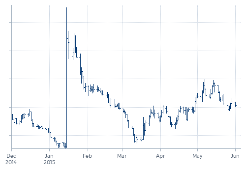
This extreme price rise which represented a 32(!) standard deviation move, has a huge impact on the measured volatility. As shown by the green line in Graph 3, the six-week daily standard deviation explodes immediately after the event by a factor of six. And six weeks later, it falls again by a factor just a little less than that. This abrupt fall six weeks after the event, essentially assuming that every price move becomes completely irrelevant after six weeks (or any other fixed time period), can easily be solved if we change from linear estimation over a fixed period to exponentially decaying estimation.
This is shown by the orange line in the graph. With an exponentially decaying volatility estimate, a new observation is weighted the same as in a linear estimate, so the orange line jumps up with roughly the same factor six as the green line. But after that, its weight (read: importance) in the calculation of the estimate immediately starts to decay, ultimately getting close to zero.
Graph 3: Different volatility estimates for Swiss franc / U.S. dollar
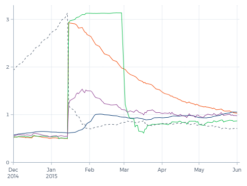
This clearly makes a difference. The arbitrarily timed drop of the estimate, such as in the green line, is gone. But is it an improvement? For risk management purposes we do not want to describe the (recent) past, but make a reasonable projection of the future. If we would have the benefit of hindsight, then we could do so by measuring the future standard deviation.
The dotted line shows the exponentially backwards decayed future standard deviation. How well do the measured historical standard deviations (the green and orange lines) serve as predictors of the future (the dotted line)? Moving towards the price explosion in response to the SNB-step, this ideally projected standard deviation rose steadily, but understandably the measured historical standard deviations did not foresee this explosion at all. However, immediately after the price jump, the future standard deviation is significantly lower than the measured historical ones. Now the fall of the green line after six weeks does not seem so bad at all; it falls back to the level where it should be, while the exponentially smoothed version keeps on overestimating for a few more months. But in the first six weeks after the jump, both estimators heavily overestimate the future volatility.
Second moment measures
This is a well-known phenomenon in statistics. Standard deviation and Pearson correlation are so called second moment measures, meaning 'averages of squared numbers'. A disadvantage of such measures is that they tend to be instable, as shown by Graph 3. The consequence is that they serve as very poor estimators. This instability gets even worse when we are dealing with leptokurtic distributions (which display a high peak and fat tails), which is typically the case with returns in financial markets. When measuring standard deviation, a series of observations in the high peak of the distribution (i.e. days with little price movement) will lead to an underestimation of the real standard deviation, while the occurrence of a fat tail event will lead to an overestimation.
We can bypass a large part of this problem if we use a first moment volatility measure instead of a second moment one. The purple line in Graph 3 shows an exponentially smoothed first moment estimator for the standard deviation.
In normal market environments, the purple line and the orange line stick closely together. But as the graph shows, the sensitivity to a large price move of the first moment estimator is significantly less than of the second moment estimator. While the second moment estimators increase with a factor of six, the first moment estimator increases with a factor of only 2.5. Still overshooting the future standard deviation, but to a much lesser extent.
The standard models were designed for the non-crisis periods and they have proven quite successful in that context.
A further step could be to use an estimator based on a volatility measure that is kurtosis-insensitive. The blue line is an example of such an estimator. It barely rises on the price explosion. In this illustration, the blue line underestimates the volatility the first two weeks after the jump. On the other hand, it produced the highest estimation before the jump. In the graph, the difference may not seem like a lot, but such a 25% higher estimation of the volatility before the jump would reduce the loss on the trade by as much as 20%, or would represent the difference between a 32 standard deviation-move and a 26 standard deviation-move.
Transtrend's position
Our risk management has always been focused on controlling the magnitude of potential losses due to extreme events. Our guiding principle is that this should be done by anticipation, not by response. We acknowledge and have experienced that in extreme events, trading out of losing positions is not possible, or only at the cost of paying a large liquidity premium. To avoid this, the position sizes and the real diversification in investment portfolios should always be such that an immediate liquidation of positions after a sudden large market move is not necessary. Using lower moment estimators for higher moment statistics is just one of the chosen techniques to accomplish this.
Transtrend typically does not sell in sell-offs and does not buy in sharp rallies. As such, we do not contribute to the systemic risk mentioned above. However, that does not mean that our trading programs are immune to this systemic risk. And not contributing surely does not make that risk disappear. To reduce such a systemic risk requires different investors to use different risk management techniques, tailored to their specific investment strategies, and preferable without using higher moment estimators. A less rigorous application of VaR limits would also help the stability of markets.
- Source of price and risk data used in all graphs in this article: Thomson Reuters, Bloomberg and Transtrend.