- A high kurtosis is more often caused by processes that directly contribute to a 'high peak', than by processes that directly contribute to 'fat tails'.
- Trend following strategies are usually able to benefit from these 'fat tails'.
- The unavoidable flipside is that trend following strategies usually struggle to generate positive returns in 'high peaks'.
An interesting way to study markets is from the perspective of kurtosis. As most people know by now: a larger kurtosis leads to ‘fat tails’, which can be fatal when underestimated. How can the behavior of markets be viewed in the context of kurtosis? And can this potentially explain the somewhat disappointing results of trend following strategies in the last few years?
On peaks and tails
A multiple choice question
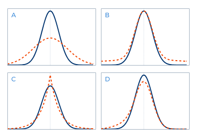
When kurtosis is the subject of conversation, most people acknowledge the major importance of ‘fat tails’, but only few really comprehend the underlying processes. The four graphs each show two probability distribution functions. The blue curve each time represents a Normal distribution. In one of these graphs the orange curve represents a distribution with exactly the same standard deviation as the blue curve, but with a larger kurtosis. The question is: which graph?
The orange curve in Graph A actually just shows a Normal distribution with a larger standard deviation. In graph D the difference lies in another statistic: skewness. Here the distribution is (negatively) skewed, which is also very relevant for risk management, but which is separate from kurtosis.
Graph B does show obvious fat tails, but statistically it does not make any sense. The surface below the orange curve should be equal to the surface below the blue one. Because if the probability of a ‘large move’ is higher, the probability of a different move should be lower. But which ‘different move’? Not the probability of a ‘small move’, because that would bring us back to graph A, i.e. simply a higher standard deviation. A higher kurtosis always goes hand in hand with a higher than ‘normal’ probability of both a ‘large move’ and ‘small move’, in combination with a lower than ‘normal’ probability of a ‘medium-sized move’. This is exactly what is depicted in graph C.
A high kurtosis is more often caused by processes that directly contribute to a high peak, than by processes that directly contribute to fat tails.
The biggest misconception with respect to a high kurtosis is that many people concentrate completely on the ‘fat tails’ and ignore the ‘high peak’. While these fat tails would not be there without the high peak. In fact, a high kurtosis is more often caused by processes that directly contribute to a high peak, than by processes that directly contribute to fat tails. High on the list of infamous drivers of high peakedness are numerous well-intended measures that aim to reduce risk. So the first conclusion should be: if we wish to protect ourselves against the impact of fat tails, we have to be wary of high peaks.
An exchange of standard deviation for kurtosis
A simple thought experiment can give a bit more insight into the relationship between high peaks and fat tails, and the associated interaction between standard deviation and kurtosis. Imagine that you own stocks in company X. You perform your risk analysis on historical daily returns of the stock. But one morning you realize that these return series do not include the Saturdays and Sundays. Although there is no trading in the stock on these days, does this mean they should be ignored? You decide to add them to your return series, using a return of 0%. Which effect does this have on the standard deviation of the daily returns? By adding all these ‘low volatile’ weekend days, it will become lower. A lot of people would say that the risk of this investment also declines. But risk and standard deviation are not the same thing. In this case we are still dealing with precisely the same stock, and therefore with precisely the same risk.
Volatility or standard deviation?
In literature on investing often ‘the volatility’ is mentioned when really the standard deviation is meant, or the standard deviation is calculated when the goal is to know the volatility. In general, volatility means variation of price, which can in principle manifest itself in standard deviation as well as other forms of variation. In this article we stick to the term standard deviation. Especially when dealing with a high kurtosis, the difference between standard deviation and volatility becomes relevant.
So we now have a return series with a smaller standard deviation, but with the same risk. Where does the ‘missing’ risk hide? Precisely: in a higher kurtosis. All these 0% return days form a high peak. When continuing to apply the Normal distribution, this peak pulls the distribution ‘inward’ (i.e. the standard deviation downwards), causing the returns on the outsides to now overshoot the Normal curve. There we have our fat tails.
This is in fact the exchange of standard deviation for kurtosis. The risk stays the same, but through the lower standard deviation it is more treacherous. It’s hidden in the higher kurtosis. Remember we did not increase the kurtosis by a direct addition of tail-risk, but by adding an (in itself not dangerous) high peak. Not being alert to this phenomenon, may give a false sense of security.
The interaction between deviation and kurtosis is well known in building engineering. The top floors of high-rise buildings sway a couple of meters when it storms. One could easily construct buildings that are less flexible. But these would not be safer. During earthquakes the least flexible buildings are the first to collapse. Every now and then a ‘resident’ may complain about this scary swaying, but no architect will take this complaint seriously.
In principle, similar laws as in building engineering apply to the economy. Here also, movement (manifesting itself through standard deviation) is healthy to prevent disaster (in the form of fat tails). Such healthy forms of movement include: that countries or companies that structurally do not have their house in order default. That diverging economic developments in two countries result in a movement of their exchange rate, or in a movement of capital or labor in case these countries share the same currency. That unhealthy economic sectors are restructured, even if this causes lay-offs.

The interaction between deviation and kurtosis is well known in building engineering. The top floors of high-rise buildings sway a couple of meters when it storms. One could easily construct buildings that are less flexible. But these would not be safer.
These forms of movement understandably are also subject to criticism from ‘residents’. But unlike in building engineering, the ‘architects’ in the economy (like politicians) are sensitive to this criticism. They resort easily to measures that contribute to peakedness. To forms of intervention that bring stability in the short term, but that are impossible to sustain indefinitely. Certainly not globally. Not all countries can stimulate their exports with a weak currency. Government debt cannot keep rising without any consequences. Effective yields cannot stay negative forever. Quantitative easing policies in principle lower standard deviation, but at the same time contribute to higher kurtosis.
Investing in the presence of kurtosis
Investors who look at stock markets in for example 2009 and 2012 from a classical perspective, might consider themselves in investor’s paradise: nicely rising stock markets with a low volatility. But investors who look at these markets from a kurtosis perspective notice the typical symptoms of high peakedness and are not lulled into a false sense of security by treacherously low standard deviations. They recognize a sign of potential fat tails.
The good news for such investors is that trend following strategies usually are able to benefit from these fat tails. The unavoidable flipside of this trait is that trend following strategies usually struggle to generate positive returns in high peaks. There are two explanations for this. The first lies in the low standard deviation in such environments. We believe that the ultimate source of sustainable returns of virtually all investment styles is the harvesting of risk premium. Market participants looking to unload price risk will – directly or indirectly – pay a premium to market participants willing and able to absorb this risk. The higher the perceived risk, the higher the premium. When, however, governments (e.g. through central banks) absorb such risks for free – or at least give that impression – this risk premium will be significantly lower. Who, after all, will pay a premium for insurance against a natural disaster, when (the impression exists that) the government will compensate for any damages anyway!
We believe that the ultimate source of sustainable returns of virtually all investment styles is the harvesting of risk premium.
The second explanation for the lack of performance during high peaks applies specifically to trend following strategies and lies in another statistical phenomenon: autocorrelation. Classical efficient market economists assume that successive price changes are uncorrelated. Trend following strategies operate contrary to this principle, as they anticipate forms of positive autocorrelation, meaning that after a rise markets have a tendency to keep rising (and vice versa). We do not believe however, that markets consistently exhibit positive autocorrelation. From a kurtosis point of view we recognize symptoms consistent with periods of positive autocorrelation alternated by periods of negative autocorrelation. The latter ones are periods when markets have a tendency to decline after a rise (and vice versa).
Such an alternating sign of the autocorrelation of, for example, daily returns expresses itself in a higher kurtosis of, for example, the weekly returns (see boxed text below). Periods with positively autocorrelated daily returns exaggerate the fat tails in the weekly and monthly returns and periods with negatively autocorrelated daily returns exaggerate the high peak. Many ‘stabilizing’ government interventions are negatively (auto)corrective by nature: when according to the government a market moves too much in one direction, an intervention takes place to turn the tide. This way it magnifies the high peak in the lower time dimensions (such as weekly or monthly returns). At the same time it is not favorable for trend following strategies that thrive on positive autocorrelation.
Mixed distributions
Let σ denote the standard deviation of daily returns. If consecutive returns are independent, so not autocorrelated, the standard deviation of the weekly returns would equal √5∙σ (assuming every week has 5 trading days).
If there is positive autocorrelation, the standard deviation of the weekly returns is higher than √5∙σ. In extremis, if after each positive return, the market would rise just as much the next day, the standard deviation of weekly returns would equal 5∙σ.
If there is negative autocorrelation, the weekly standard deviation is lower than √5∙σ. In extremis, if the autocorrelation is perfectly negative, it simply equals σ.
So if there are alternating periods with positive and negative autocorrelations in daily returns, this gives alternating periods with higher and lower standard deviations in the weekly returns. We are dealing here with a higher kurtosis caused by ‘mixed distributions’, where the periods with the higher standard deviation cause the fat tails and the periods with the lower standard deviation cause the high peak.
And with that we have also explained why trend following strategies generally perform well in the fat tails. They are then able to profit from the positive autocorrelation that (also) causes the tail. These are exactly the circumstances in which trend following strategies perform the best. Note that we specifically mean fat tails in the lower time dimensions, in particular in the monthly returns. If the fat tail lies in the daily returns themselves, meaning a ‘large move’ in one or two days, then this is just as treacherous for a trend following strategy as for any other longer term investment strategy. A trend follower should therefore be particularly concerned about limiting the impact of these types of ‘jumps’ and keep in mind that positions should always be ‘tail-proof’.