Updated: July 2023
- As of January 2018 we are required to report transaction costs, including implementation costs, according to the PRIIPs methodology.
- This methodology does not meet the basic premise that buying at a higher price is more expensive than buying at a lower price. Even selling in a flash crash will not necessarily result in high implementation costs to be reported.
- Transtrend regards good execution to be an essential ingredient of any investment strategy; we will continue to closely examine all execution of our trading programs in a sensible way.
PRIIPs and MiFID II prescribe that investors must be provided with information about costs and charges of investment products and investment services.¹ One element of this costs and charges disclosure is the disclosure of ‘actual transaction costs’, which include implementation costs. PRIIPs describes in detail how these actual transaction costs must be calculated and ESMA implies that this method must also be applied when calculating costs and charges for certain MiFID II services.²
Buying and selling some Amazon stock
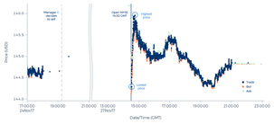
Suppose an investor is interested in Amazon. He has read a lot about the firm and has high expectations of the business Amazon is involved in. On 27 March 2017 he notices that Amazon stock is trading on Nasdaq at $835 per share. He thinks that this is a good opportunity to buy the stock. So he sends an order to his broker to buy the stock ‘at best’. This turns out to be a good investment decision. One month later, on 27 April, after Amazon presents strong quarterly results, the investor witnesses the stock trading above 952. He feels that this is a good moment to take profit on his investment. So he immediately instructs his broker to sell the stock on the Nasdaq opening on 28 April. Confident about the success of his investment, the investor takes a look at the account statements that he receives from his broker. But he is a little disappointed to see not the 14.0% profit on his investment that he had expected to find – the rise from 835 up to 952 – but rather a profit of only 12.9% instead. The difference is only to a minor extent explained by the commission that he had to pay to his broker. More important are the prices that the broker traded for him. As it turns out, in March he bought at 837 instead of 835. And in April he didn’t sell at 952, but at 945.
Graph 1: Amazon stock on 27/28 April 2017
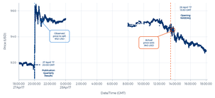
This difference between the prices that an investor might have expected to trade at and the prices that he actually pays or receives, are generally referred to as ‘implementation costs’. According to MiFID II, brokers and investment managers have to make such costs transparent to their investors as part of the transaction costs. Looking at the calculation method of these costs according to PRIIPs, this seems to be straightforward in the above example. At the basis lies the ‘arrival price’, which is normally the price of the stock at the moment (‘arrival time’) that the order is sent to another person, in this example to the broker. The difference between the prices actually traded and the arrival price should be disclosed as part of the transaction costs. In this example that would be $2 on 27 March (837 minus 835), and $7 on 28 April (952 minus 945). And these numbers indeed fully explain the investor’s level of disappointment in this example.
It is important to note that these implied implementation costs cannot simply be attributed to the broker’s skills. In this example, if the investor had sent his order to buy on 27 March not ‘at best’, but at a limit of 835, the broker would not have bought at any price above 835. And in the situation of 28 April, it was the order to sell on the Nasdaq opening that precluded the broker from selling at 952. If the investor had wanted to sell at 952, he should have instructed his broker to start selling at 952 or better immediately after receiving the order, instead of instructing the broker to wait until the Nasdaq opening the next day.
One might hope that this example is not a common occurrence. This investor was sending orders to his broker without a price limit, effectively instructing him to buy and later on sell Amazon stock at any price. If all investors were to submit such unconditional orders, markets would not function. Market equilibrium can only be reached, if there is a price level below which fewer participants are willing to sell and above which fewer participants are willing to buy. It is the responsibility of all market participants to make this happen, by only submitting orders with a decent price limit.
If the investor is a private investor submitting orders to a professional broker, one could argue that this responsibility to tie a reasonable price limit to orders sent to the market lies in the broker’s hands. The duty to report transaction costs including implementation costs could help raise brokers’ awareness of this responsibility. However, assuming that the broker selling on 28 April in the above example calculates those transaction costs according to the PRIIPs method, the broker will very likely not report $7 transaction costs. He will probably use an ‘arrival price’ that corresponds with the prices traded around the opening, as this was the time that the order was executed. This is because PRIIPs describes that where an order is executed without being transmitted to another person, as is the case from the broker’s perspective in this example, the arrival price should be determined as the mid-market price of the investment at the time when the transaction was executed.³ This would result in lower reported transaction costs. And for good reason, we would argue, as the investor specifically instructed the broker to sell at the Nasdaq opening.
However, if the investor in this example had been an investment manager trading on behalf of his clients, then according to the PRIIPs methodology, this investment manager would have had to report the transaction costs exactly as described in the example.
The basic premise of measuring transaction costs should be that buying at lower prices results in lower transaction costs to be reported than buying at higher prices does.
So, in this example, an investor who trades directly through a broker will get reported lower transaction costs than he would get reported by his investment manager if this investment manager would do exactly the same trade on his behalf, trading at exactly the same prices. This may seem strange at first. But we believe there are good grounds for this difference. As explained above, one could argue that while the responsibility to trade against reasonable prices lies in the hands of the executing broker, the broker is bound by the limitations that the investor imposes on him. In the case of investment management, it is indisputably clear that the responsibility for trading at reasonable price levels lies fully in the hands of the investment manager. That is what the investor has hired him to do. So the investor may expect transparency from his investment manager showing whether or not he has succeeded in fulfilling this responsibility.
It would be commendable if the transaction costs reporting according to PRIIPs were to offer this transparency, but unfortunately, it does not. The basic premise of measuring transaction costs should be that buying at lower prices results in lower transaction costs to be reported than buying at higher prices does. However, in their zeal to prescribe a generally applicable objective measurement, the writers of PRIIPs came up with such painstaking detail in their technical description, that somehow the basic premise was lost in translation. Some examples will illustrate this.
A Live Cattle example
Suppose three different investment managers are offering a similar investment strategy. On the morning of 21 November 2017, they all decide to buy the Dec’17 futures contract Live Cattle traded on CME. Each chooses a different way to execute the order:
- Manager A immediately sends an order to an executing broker instructing him to buy the contract at a limit price of 117.25 cents per pound, starting to work this order in the opening auction. Ultimately, the opening auction results in an opening price of 117.4, resulting in no fill on this order. However, a little later Manager A does get filled on his bid at 117.25.
- Manager B also immediately sends an order to an executing broker to buy the contract. But he instructs him not to work the order in the opening auction, but to await the opening price that results from that auction, and subsequently to buy the contract with the opening price as a limit. Following this instruction, the broker buys at 117.35.
- Manager C believes that the best liquidity can be found around the settlement time of the contract. He waits until 45 minutes before settlement, and then he sends an order to his broker to buy the contract at the settlement. Ultimately the contract settles that day at 117.975; and the broker buys the contract at 118.
Now look at the transaction costs that each of these three investment managers will have to report to their investors according to PRIIPs. As before, this depends on the ‘arrival price’, the price of the investment at the time when the order is transmitted to the broker.⁴
Graph 2: Live Cattle December 2017 futures contract on 20/21 November 2017
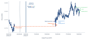
- Manager A participated in the opening auction. According to PRIIPs⁵ this manager then cannot use the opening price as the ‘arrival price’. He has to use ‘the mid-price immediately prior to the auction’ instead, which was the settlement price of 20 November in this case. Buying at 117.25 then means transaction costs of 0.15 (the difference between 117.25 and 117.10).
- Manager B did not participate in the opening auction, so he is allowed to use the opening price (117.4) as the ‘arrival price’. His order was filled at 0.05 lower, meaning transaction costs of minus 0.05.
- When Manager C sent his order to the broker, Cattle was trading at 118.25. So at 118, he bought 0.25 below that ‘arrival price’. He will report minus 0.25 transaction costs on this trade.
So the manager buying at the lowest price will report the highest transactions costs. And the manager buying at the highest price will report the lowest (even negative) transaction costs! This cannot be how this regulation was intended to work. Nor does this afford the investor any meaningful transparency.
The transaction cost measurement according to PRIIPs is defined around the ‘arrival price’. But this ‘arrival price’ constitutes no relevant benchmark whatsoever in the relationship between an investor and his investment manager.
What is going wrong here? The transaction cost measurement according to PRIIPs is defined around the ‘arrival price’. This ‘arrival price’ differs depending on whether or not an order is ‘transmitted to another person’ and at what time this is done. But this ‘arrival price’ constitutes no relevant benchmark whatsoever in the relationship between an investor and his investment manager. The investment manager does not receive orders from his investors that he should execute the best way that he can from the time that he receives those orders. The investment manager trades on behalf of his investors, making all trading decisions at his discretion. The decision whether or not to ‘transmit an order to another person’, and if so, the decision when to ‘transmit the order to another person’, are just as much a part of the investment manager’s trading strategy as the decision at what price to buy or sell. And this integrated set of decision processes as a whole determines whether the investment manager buys at a low price, as our Manager A did, or at a high price, just like Manager C. For the prices that the investor pays, the ‘arrival price’ from the PRIIPs methodology has no relevance at all. So why use it in calculating transaction costs? This does not offer the investor any transparency as to how well his investment manager implemented its trading strategy.
Investment decisions and trade execution should be considered integrated processes. Any attempt to rate one process without regard to the other is doomed to be meaningless.
To complicate matters even further, an investment manager does more than execute trades: he executes an investment strategy. He decides not only at which moment and at which price to buy, as described in the paragraph above, but he also decides whether to buy or to sell in the first place. In traditional investment theory, all of this constitutes just one decision. A rational investor doesn't decide to sell; he decides that he is willing to sell above a certain price level. For markets to function, it is necessary that not only investors willing to buy or sell at the current price express their willingness to trade, but that also investors willing to sell above the current price and investors willing to buy below the current price transmit this information to the market. Otherwise, no equilibrium would be reached. So the only indivisible trading activity of an investment manager is to bid at the price level he is willing to buy and/or to offer at the price level he is willing to sell. Therefore, investment decisions and trade execution should be considered integrated processes. Any attempt to rate one process without regard to the other is doomed to be meaningless.
The most expensive type of execution we can think of is selling in a flash crash. As an investor, you might expect that such a needlessly expensive execution will be made transparent in the reporting of high transaction costs. Under PRIIPs this is however not necessarily the case: not in the reporting done by an executing broker who does not transmit the order to another person (since he will most probably calculate the transaction costs relative to the low mid-price in the flash crash)⁶, nor in the reporting done by the investment manager, as the following example will illustrate.
Trend following in COMEX Silver
Consider two investment managers who both offer a trend following strategy. Each manager holds a short position in the Sep’17 contract COMEX Silver, which each of them entered on 5 July at a price of 1600 cents per troy ounce. On the evening of 6 July this futures contract collapses, to the extent that COMEX’s ‘velocity logic’ functionality automatically holds trading for 10 seconds. At that moment, the contract trades at 1471.5.
Manager D follows the market closely. In his opinion, the market has broken an important break-out level in its steep decline, so he regards this to be a good opportunity to sell more contracts. He sends an order to his broker, instructing him to sell another 200 contracts starting immediately after the 10-second break, using a VWAP-strategy without a price limit.
Manager E follows the market closely as well. In his view, the market behaves like a typical disrupted market, trading well below its fair value. He sends an order to his broker to buy 200 contracts starting immediately after the 10-second break, using a fairly aggressive execution strategy, with a price limit at 1525 attached. This will liquidate his entire short position if filled.
Suppose both managers end up trading against each other. Their execution starts at a price level as low as 1434, but within a minute the price they trade at rises to 1525. At that moment both are filled on their order. Their average traded price is 1485. As it turns out, Manager E seems to have judged the situation correctly. The price of silver continues to rise. For the remainder of that day, the contract does not trade below 1525. And before the end of the month, it is trading above 1650 again. At that level Manager D liquidates his short position.
Which transaction costs will they report? The ‘arrival price’ for both is 1471.5. And both managers executed on an average price of 1485. So Manager E, who gauged the situation correctly and helped to bring this disrupted market back up towards its fair value with his aggressive buying – making a profit for his investors on his short trade in doing so – will have to report ¢13.5 transaction costs on this trade. Manager D on the other hand, who misjudged the situation and further disrupted the market with his aggressive selling – losing money for his investors with his actions – can proudly report minus 13.5 transaction costs.
Trend following in COMEX Silver - continued
Then the situation takes yet another turn. After the exchange is alerted to the disruption, it sees fit to adjust all prices traded below 1554 up to 1554. This means that all of the prices that Managers D and E traded were adjusted to 1554.
Graph 3: COMEX Silver September 2017 futures contract on 6 July 2017
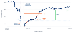
The aggravating consequence is that Manager E has to report 82.5 transaction costs. But what about the investors of Manager D? Do they gain any real transparency by getting reported minus 82.5 transaction costs? We would argue that these investors would deserve an extensive letter from their investment manager explaining that he made an error selling in a disrupted market, and that he was very lucky not to be punished for it, even getting his prices adjusted when he deliberately sold at those low prices.
What this example shows is that the PRIIPs transaction costs measure not only lacks the basic premise that ‘buying at a low price is better than buying at a high price’, but it also does not promote investment managers contributing to well-functioning markets. It even contains a disincentive to do so.
The PRIIPs transaction costs measure does not promote investment managers contributing to well-functioning markets. It even contains a disincentive to do so.
Let us have another look at the Live Cattle example. Both Managers B and C were effectively submitting an order to buy at any price. Manager B may have given the price set in the opening auction as a price limit, but at the moment of submitting his order, he didn’t know what that opening price was going to be. If the opening auction had resulted in an unreasonably high price, Manager B would have been just as willing to buy at that high price. The only manager in this example who contributed to a well-functioning market was Manager A. He is the one paying the lowest price, and yet he is the one who has the highest transaction costs to report.
The order submitted by Manager B may sound a little strange, but this is exactly the kind of order investment managers are encouraged to submit if they try to limit the transaction costs to be reported according to PRIIPs.⁷ This does not necessarily serve the investor’s best interests. It is a strategy that is aimed at minimizing transaction costs, not at buying at a low price. And it doesn’t serve the functioning of the market. If investment managers refrain from contributing to the equilibrium process in the opening auction, which process will then establish a meaningful opening price?
And if an opening price is not meaningful, why should PRIIPs treat it as if it is?⁸ The references that this regulation makes to the opening price do not seem to be founded on the dynamics of modern markets. It sounds reasonable if one thinks of a market where all trading takes place on one platform. That platform is closed during the night, and when it opens, preferably with a well-functioning opening auction, there is immediately good liquidity. A market like CME Live Cattle would match most of these conditions. However, nowadays, such a market is the exception rather than the rule. Two more common examples:
An opening auction example
On CME screens futures contracts are traded on various S&P stock indices. These screens are open 23 hours a day. After the close of the screen on Friday 8 December 2017, Manager F decides that he is willing to sell up to 16 contracts S&P Financial Index expiring in December 2017 at a limit price of 343.8 and that he is willing to buy up to 10 contracts at a limit of 329.75. He transmits both orders to the exchange through his broker using a smart execution algorithm.
The regular trading session of the S&P index futures starts Sunday night at 23:00 GMT following a 15-minute opening auction. In the case of the Financial Index, the auction did not result in an opening price, but in a bid and offer with a spread of more than 4 percent between the two. There just wasn’t enough liquidity. The first trade in the screen is set around 9:33 GMT, traded at 337.4. Almost immediately after that, Manager F gets filled on 3 of his 10 contracts bid at 329.75. From the opening of the NY-stock market at 14:30 GMT, the Financial Index futures becomes much more liquid. Around 14:57 GMT Manager F gets filled on his 10 contracts offered at 343.8.
Graph 4: E-mini Financial Select Sector December 2017 futures contract on 8-11 December 2017
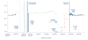
In a case like this, the determination of the ‘opening price’ is entirely arbitrary. For instance, one could choose to use the average of the bid and the offer at the end of the opening auction to represent market price. However, this assumes that the best offer is just as accurate as the best bid. With liquidity so low, when the spread between bid and offer is so wide, that assumption is not founded. And also the first price actually traded doesn’t seem representative of the market price; in our experience, when a market opens trading like this, the first price traded is often an outlier.
A wide opening range
Cash stocks listed on NYSE and Nasdaq start with an official ‘on exchange’ opening at 14:30 GMT. However, these stocks can be traded, both on and off exchange, prior to that. In some stocks this takes place regularly. In most U.S. stocks the real trading starts ‘at once’ from 14:30GMT onwards, but not at a meaningful equilibrium price. The price range set in the first minutes of trading often makes up a significant part of the entire day range. Suppose Manager G sells some McKesson Corp stock around the opening of NYSE on Monday 27 November. How should we assign a meaningful ‘transaction cost’ to his fills?
Graph 5: McKesson Corp stock on 24-27 November 2017
Our simple rule would state: selling above 145.5 is good; selling below 145 is expensive, irrespective of the level of the ‘on exchange’ opening, irrespective of whether the trade is executed on exchange or off exchange, irrespective of whether the trade is executed ‘at the opening’ or somewhat earlier or later, and irrespective of at what time before the opening the order was transmitted to another person. But again, this is not how PRIIPs values it.
Prices move. The execution of orders impacts that movement. In fact, order execution is the only force making market prices move. These price moves impact investors’ returns, including those investors whose orders are executed in these moving markets. It is good that investors are aware of this. But the idea that this price impact can be measured as a cost in an objective and meaningful way is rather naïve. The PRIIPs methodology does not achieve that purpose in many commonly occurring scenarios. And that is why this measure fails to offer investors any real transparency.
Isn’t there a better way? We think there is. Investment managers such as Transtrend are in essence trading managers. They are hired to buy and to sell markets. The returns of the trading strategy are determined by the difference between the prices at which the trading manager buys and the prices at which he sells. If the trading manager buys at a higher price, one could have a discussion whether this means his transaction costs are higher or his trading returns are lower, but any such discussion is fruitless. The effect is the same. Transaction costs are nothing but the mirror image of trading returns. And trading returns can be measured in a uniform and indisputably transparent way: sell price less buy price. And yes, to calculate the net investment returns, all costs that are clearly attributable costs, such as broker commissions, must be subtracted from these trading returns.
Transtrend regards good execution to be an essential ingredient of any investment strategy; we will continue to closely examine all execution of our trading programs in a sensible way.
Transtrend’s position
From January 2018 we are required to report transaction costs including implementation costs. We will however clearly distinguish between costs and charges actually paid to third parties for the execution of trades (e.g. broker commissions and exchange costs), and ‘implementation costs’. Together, these will constitute the ‘actual transaction costs’ as described in PRIIPs.
For some of the funds for which we are appointed as AIFM, we have to provide the PRIIPs-related information to retail clients invested in these funds; for our managed account clients MiFID leaves some room for using a different methodology. This would allow us to report two different sets of transaction costs for what are essentially the same transactions, derived from the same trading program, executed in the same way, at the same price, only because they were done for two different types of accounts. We do not think that transparency is served if we were to do so. That is why we have chosen to apply the PRIIPs methodology for all accounts, in spite of our conviction, amply substantiated above, that the resulting figures are not particularly meaningful.
As the above examples illustrate, the PRIIPs methodology cannot be applied without making certain assumptions. Below, we describe the assumptions made by Transtrend in order to calculate the transaction costs according to PRIIPs.
In our execution, orders are often split into various ‘child orders’, and our traders have different ways of working these orders. A part of the order can be sent to a broker at some point in time or traded directly with a counterparty. We do not think it is in line with the ideas behind PRIIPs if different fills on essentially the same order, or different choices made in the execution of a single order, are compared with different arrival prices. That is why we have chosen to tie one uniform arrival time, and therefore a uniform arrival price, to every individual order, irrespective of the moment that a specific part of the order is eventually executed (whether via transmission of the order to another person or not). This arrival time is tied to the order at the moment that our trader tags the order as ‘ready to be worked’. Execution cannot start earlier than that. As a consequence, in the Live Cattle example above, the orders transmitted by Managers A, B, and C would all get the same arrival time and arrival price: the arrival time and price described for Manager A.
In our execution, we typically act as a liquidity provider. We only work limit orders, usually bidding below and/or offering above, recently traded prices. With these orders we also participate in opening auctions and during illiquid trading hours. In the above examples, the orders worked by Manager F in the S&P Financial Index were actual orders and fills from our Diversified Trend Program. And as Manager G we sold McKesson Corp at 145.96 for our Equity Trend Program. In our interpretation of PRIIPs the fact that we participated in the price discovery process means that we cannot use the ‘opening price’ in calculating our transaction costs.⁹ So we have determined that we will never use the ‘opening price’ for this purpose. Instead we will use a price that is representative of the last liquid trading moment before the market closed as the arrival price. We will do this not only when orders are tagged as ‘ready to be worked’ when the specific market was closed, but also when this is done at a moment that there is no meaningful liquidity in a market. For transactions like the ones mentioned in the S&P Financial Index and in McKesson, this will typically result in negative ‘implementation costs’.
The majority of the transactions that we execute for our Diversified Trend Program are part of synthetic trades, where we trade one financial instrument against or combined with another financial instrument. For example, we could buy German Bund on EUREX while selling U.S. Treasury Notes on CME. PRIIPs states that the transaction costs when trading such a customized instrument shall be calculated with reference to the underlying assets.¹⁰ So that is how we will calculate them. As a consequence, if an order in such a synthetic is tagged as ‘ready to be worked’ at the moment that either one of the two instruments is closed or illiquid, the arrival price used for this leg of the trade will be set at a different point in time than the arrival price in the other leg. This will likely result in a meaningless implicit arrival price for the customized instrument that we are actually executing.
Our investors should be aware that the implementation costs we report are meaningless and offer no transparency at all. We report these figures only because we are obliged to do so. Our investors can rest assured that we will not adjust our execution just for the sake of reporting lower implementation costs. For instance, we will not deliberately avoid contributing to establishing an equilibrium in the market by starting to submit orders of the type submitted by Manager B in the example above.
However, we do consider good execution an essential ingredient of an investment strategy. That is why we closely examine all execution of our trading programs, but in a way that differs fundamentally from the PRIIPs methodology. In our daily analysis of fills, we compare the fills on all buys with the lowest relevant price traded during that particular day, starting from the close of the previous day onwards. Likewise, we compare the fills on everything sold with the highest relevant price.
Of course we do not expect that we will actually buy at what in hindsight turns out to have been the lowest price, so we will not treat it as a ‘cost’ if we paid a higher price. But we do think that such a comparison with the best possible price is the most straightforward and objective way to identify those trades that potentially may have been executed in a better way. In our analysis we do not only question the prices that we traded at, but also the reason why we traded that particular market in the first place. We also examine any trades that we did not execute but that potentially could have been executed. We do not split ‘the legs’ of an order in a synthetic market; in fact, we specifically check whether these legs have been executed simultaneously to prevent unintended execution risk. And we closely check all of our execution for signs of market disturbance.
This way of analyzing fills does meet the basic premises. Buying at a higher price will always be considered more expensive than buying at a lower price. And selling in a flash crash will be identified as extremely expensive.
Addendum — July 2023
On 1 January 2023, amendments to the PRIIPS methodology entered into force. Considering our earlier criticism, we welcomed this revision and were curious if the shortcomings we highlighted had been amended.
In its considerations, the revised regulation specifically mentions it wishes to avoid the occurrence of negative implementation costs in order to avoid the risk of confusing investors. Regretfully there have not been made any specific changes to the way the implementation costs of limit orders should be calculated; and since the existing calculation method in most cases will lead to negative transaction costs for limit orders, we doubt this goal has been reached.
Furthermore, in the amended version the arrival price of orders that are worked at a pre-determined time should be calculated at that pre-determined time. This means for instance that in our Live Cattle example, Manager C should use the settlement price as its arrival price since he specifically instructed his broker to buy the contract at the settlement. In the previous version of PRIIPS, Manager C was allowed to report the price at the moment he sent the order to the broker as his arrival price. In our scenario these amendments would have led to less divergent transactions costs (0.025 instead of minus 0.25), but it would still lack the basic premise that ‘buying at a low price is better than buying at a high price’, since Manager A pays the lowest price but still has to report the highest transaction costs.
In our article we also discussed the fact that PRIIPS obliges market participants to choose an arrival price that does not adequately reflect the market price level when there is no mid-market price available. This issue has been partially addressed and market participants are in these instances no longer expected to use the opening or closing price but should use the most recently available price as their arrival price instead. This approach is in line with Transtrend’s calculation method of using the most recently available price at the most recent liquid trading moment as its arrival price.
In conclusion, although the changes offer some improvements, overall the regulation still does not fulfill its ultimate goal — i.e., provide investors with a meaningful insight into the quality of the service they are receiving.
- Source of price data used in all graphs in this article: Thomson Reuters, Bloomberg and Transtrend.
Footnotes
¹ PRIIPs: Regulation (EU) No 1286/2014 article 8 paragraph 3(f) as further described in Commission Delegated Regulation (EU) 2017/653 article 5 and Annex VI to this Delegated Regulation, article 12 – 23.
MiFID II: Directive 2014/65/EU article 24 as further described in Commission Delegated Regulation (EU) 2017/565 article 50.
² ESMA Questions and Answers on MiFID II and MiFIR investor protection and intermediaries topics, dated 18 December 2017. Chapter 9, a.o. question 8 and 12.
³ Annex VI to the Commission Delegated Regulation (EU) 2017/653, article 14.
⁴ According to the Questions and Answers on the PRIIPs KID dated 18 August 2017, question 53, orders that are limit orders should not be treated differently to other orders when determining the arrival price.
⁵ Annex VI to the Commission Delegated Regulation (EU) 2017/653, article 18.
⁶ Annex VI to the Commission Delegated Regulation (EU) 2017/653, article 14.
⁷ Annex VI to the Commission Delegated Regulation (EU) 2017/653, article 18.
⁸ Annex VI to the Commission Delegated Regulation (EU) 2017/653, describes in various instances that the ‘opening price’ should be used as arrival price (a.o article 14 and 15).
⁹ Annex VI to the Commission Delegated Regulation (EU) 2017/653, article 18.
¹⁰ Annex VI to the Commission Delegated Regulation (EU) 2017/653, article 16(b).