Dit artikel is alleen in het Engels beschikbaar.

In the first part of this series on the sources of investment returns and how to capture them effectively and efficiently, we introduced our alternative approach:

Some sources of beta are harder to capture than others. Or, to put it differently, the harder-to-capture types of beta require more skill than the easily-captured types of beta. But despite the skill required, it all remains beta.

In this article we will discuss one of the important implications of this alternative approach to alpha and beta: the non-portability of alpha. When positive alpha cannot be acquired, the art of investing boils down to avoiding negative alpha. We will illustrate this by comparing an easy-to-capture type of beta with a harder-to-capture type of beta.

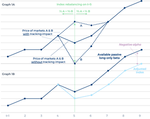
An example of an easy-to-capture beta is the beta of a passive long-only index investment. In our June 2018 article Beat the index, don’t beat the market we illustrated how the market impact of index tracking strategies that aim to capture this beta results in negative alpha dragging down the index that is tracked. The mechanism at work is depicted in the following graph, taken from that article:

Graph 1 – The negative alpha of index tracking

To explain the mechanism we assumed an imaginary index consisting of only two markets that are essentially the same: without any index tracking trading impact, their returns would be identical (the blue solid curve in Graph 1A). Because they are identical, all indices composed of any linear combination of these two markets would have the exact same returns. We further assumed that this specific index consists of one third of market A and two thirds of market B initially. On the close of the fifth day this index will be adjusted, to two thirds of market A and one third of market B. All investors tracking this index will then have to buy market A to double their position in A; and they will have to sell market B, to halve their position in B. This will have market impact: market A will close higher and market B lower as a result of the index rebalancing − we assumed by three units either way. After some time, say two days in equal steps, this temporary mispricing will be corrected, and markets A and B will return to the levels that they would have had without the index trackers’ impact (the upper and lower dashed lines in Graph 1A showing the price series of markets A and B, respectively).

To examine what happens to this index as a result of its composition adjustment, we looked at an alternative, unadjusted, index comprised of 50% in markets A and B (the dark blue curve in Graph 1B). The returns of this 50/50 index are exactly what the returns of markets A and B would have been without the impact of the investors tracking the other, adjusted index: during the mispricing the impacts on markets A and B cancel each other out in this particular combination; after the correction, any unadjusted combination of A and B will again have the same returns. The adjusted index’s returns however (the light blue curve in Graph 1B) lag the 50/50 index by a unit per the close of the fifth day, by a unit and a half per the close of the sixth day, and by two units per the close of the seventh day.

This is the direct market impact of the index tracking trading activity. One could say that the dark blue curve represents the beta of a truly passive long-only investment in these markets. An index tracking strategy achieving the returns of the adjusted index, the light blue curve, delivers this beta with a negative alpha.

Now, let’s return to the fifth day in this example. When the index tracking investors were buying market A and selling market B, other market participants must have been doing the exact opposite. These market participants must have been following a different investment strategy, for instance an arbitrage strategy. Some will call this a pure alpha strategy, but in our alternative model this is pure beta: the index trackers perceive tracking error as a risk – they pay a risk premium to avoid it. And this premium is the source of beta the arbitrageurs are after.

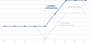
This is an example of a harder-to-capture type of beta. With hindsight it’s always clear how much beta was available in a given situation. In this example, the arbitrageur could have sold the spread (selling market A, buying market B) against a six units premium, which would have resulted in a profit of six units after a two-day holding period, as depicted by the dark blue solid curve in Graph 2.

Graph 2 – The negative alpha of an arbitrageur

The problem is, how could the arbitrageur have known beforehand that the premium would rise to six units? If he had expected it to rise to say eight units, and had worked the spread order at that level, he would not have found a buyer. In other words, no trade and no profit. If he instead had settled for say a two units premium, he would initially have ended up with a loss of four units at the end of the fifth day. Which means that, in order to ultimately cash in that two units premium, he should have been able to fund an initial loss of four units.

How mispriced can markets get before they turn more rational again? Getting this right is key to effectively and efficiently employing an arbitrage strategy. (Readers familiar with the history of LTCM will appreciate this.) In this example, according to our alternative model, every premium less than six units should be considered negative alpha. In practice, avoiding a large part of such negative alpha seems reasonably impossible, which makes the beta aimed for hard to capture.

Another factor adding to the almost unavoidable inefficiency of such a strategy is that the arbitrageur needs to have funds available when trading opportunities occur. These moments – and the ultimate potential of the opportunities – are hard to predict. The arbitrageur therefore needs to always have a certain amount of funds ready. But unused funds do not generate returns.

The light blue curve in Graph 2 shows the return of an arbitrageur who entered into the spread stepwise by equal amounts during the widening of the spread, reaching his position limit exactly when the spread was at its widest (i.e. selling the spread against an average premium of three units). This implementation is already better than what reasonably can be expected with such a strategy. So, even executed well, the strategy would incur significant negative alpha – three units in this example.

We now have defined a simple index tracking strategy that delivers the easy-to-capture beta in these markets with two units of negative alpha, and an arbitrage strategy that delivers a harder-to-capture beta with three units of negative alpha when executed well. An intriguing question is: how can investors most efficiently participate in these hypothetical markets A and B by allocating funds to these two strategies?

According to the academical portable alpha concept which is based on the standard distinction between alpha and beta, an investor can get the largest part of the potential return by allocating funds to the passive index tracking strategy against marginal fees. And on top of that he can buy the arbitrageur’s ‘pure alpha’, paying a fee that matches the skill required for effectively implementing such a strategy.

The question, then, is which part of his funds should the investor allocate to the arbitrage strategy? Suppose he decides on 20%, which leaves 80% available for the index tracking strategy. This would mean that he only gets 80% of the index return; not only on the days that the arbitrage strategy yields the aimed for ‘additional’ return, but also on the days that the arbitrage strategy yields no return due to a lack of opportunities.

Advocates of the portable alpha concept often solve this issue by assuming that the funds required for the ‘pure alpha’ strategy can be borrowed. However, borrowing additional funds just raises the amount of funds available; it doesn’t change the fundamental question of how the available funds can most efficiently be allocated. (The same holds when the additional funds would be made available through the use of leveraged instruments.)

Playing around with the various parameters in this example while adhering to reasonable assumptions about required funds reveals that it is difficult to combine both strategies in such a way that the combined return approaches the beta of the truly passive long-only investment we started with. Our alternative approach to investment alpha and beta explains this phenomenon well: the underperformance of the index tracking strategy is negative alpha caused by inefficiencies in capturing the aimed for beta offered by the markets A and B; the arbitrage strategy aims to benefit from these inefficiencies, but implementing this strategy introduces yet other inefficiencies.

This doesn’t mean that the truly passive strategy cannot be outperformed. For instance, an investor who is rather indifferent about his allocation to A or B can decide to hold whichever position in both markets. In case of inflows he can buy the cheaper one, and in case of outflows he can sell the more expensive one. On top of that, he can buy the cheaper one while selling the more expensive one whenever this will bring him closer to a predetermined soft target allocation.

This way the investor collects some arbitrage beta on top of the full truly passive long-only beta. We could introduce this style as a fancy new investment strategy with a fancy name like beta-layering. But it really isn’t. What we have just described is traditional active long-only investing. This used to be the dominant investment approach before the investment industry became gripped by an over-academicized fixation on rather abstract return drivers, gradually losing touch with some of the fundamental roles of investors such as offering liquidity.

To return to the analogy used in the first part of this series: instead of living healthy, investors have now defined health in pharmaceutical terms and allocate their funds to ‘capsules’. This is not the most efficient way of investing. And it isn’t healthy either.